.jpg)
PGA - Scoring Average Confidence Intervals (No R)
Single Mean Confidence Intervals
Single Mean Hypothesis Testing
Exploring Single Mean Confidence Intervals with Golf Data
Welcome video
Introduction
In this module, you will be exploring the concepts of single mean confidence intervals and single mean hypothesis tests using data from the 2023 Masters Tournament. The Masters is considered to be one of the greatest and most selective tournaments in the world of golf. Only the best current players or previous winners are allowed in. The winner of the Masters gets to wear the famed “Green Jacket” and return to play any year they would like at the Masters. The course the Masters is played at, Augusta National, is one of the most beautiful and challenging courses in the world. The course is known for its fast greens and tight fairways. The Masters is the first major of the year and is played in early April. The tournament is played over four days. After 2 days, the top 50 players and ties make the cut and play the final two days.
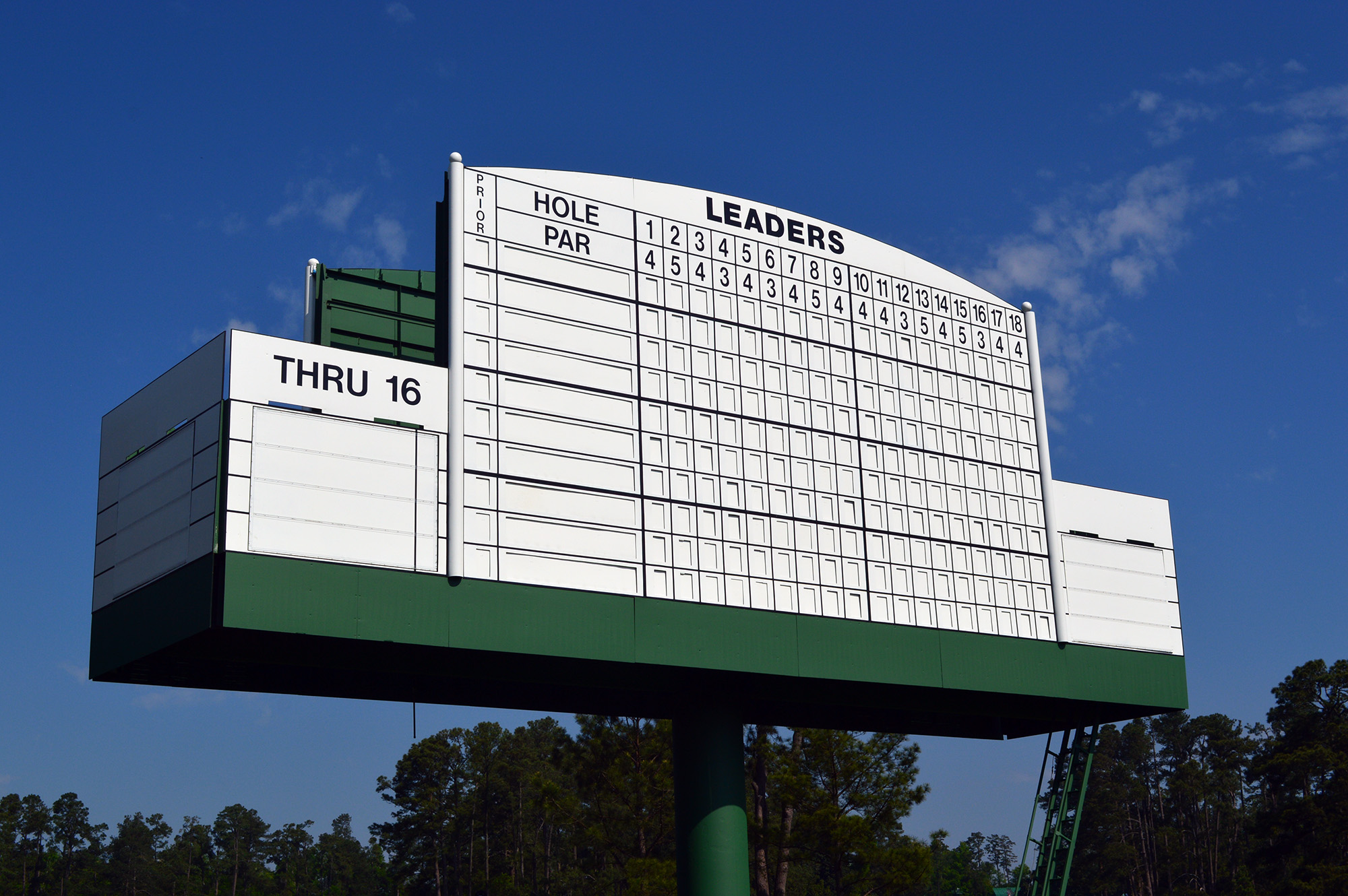
Image Source: Ryan Schreiber, CC BY 2.0, via Wikimedia Commons
View the course at Augusta National here
As mentioned before, only the best players and previous winners can compete in the tournament. With that being said, the Masters is one of the few tournaments that players from the newly created LIV golf tour can play in, although they are mostly qualifying because of their past performances at the Masters before they joined LIV golf. This leads to a mixture of regular PGA Tour professionals, LIV golfers, Amateurs, and Seniors playing in the Masters in 2023.
The focus for this module is confidence intervals and hypothesis testing for the true mean scores for different groups of players at Augusta National.
Getting started: 2023 Masters Data
The data for this lab comes from the 2023 Masters tournament. The data includes the name of golfer, the round of the tournament, the score the round, and the tour that they usually play on.
Terms to know
Before proceeding with the analysis, let’s make sure we know some important golf terminology that will help us master this lab.
Golf Terminology
- Par in golf is the amount of strokes that a good golfer is expected to take to get the ball in the hole.
- Each hole in golf has its own par. There are par 3 holes, par 4 holes, and par 5 holes.
- There are 18 holes on a golf course and the pars of each of these holes sums to par for the course, also known the course par.
- A round in golf is when a golfer plays the full set of 18 holes on the course.
- In most professional golf tournaments, all golfers play 2 rounds, the best golfers are selected and those golfers play 2 more rounds for a total of 4 rounds.
PGA Tour vs. LIV Golf
Click here to read about LIV golf’s founding and its continued impact on the PGA tour.
Single Mean Confidence Intervals
Single mean confidence intervals give a range of numbers that we can feel confident that the true population mean falls between. In the most accurate sense, a single mean confidence interval is a range of values that, if we were to take many samples and calculate the confidence interval for each sample, a certain percentage of those intervals would contain the true population mean. Because of what a single mean confidence interval is, it is innaccurate to say that there is a 95% chance (if we were constructing a 95% confidence interval) that the true mean falls within the the confidence interval. The true mean is a fixed value, so it either falls within the interval or it does not. The 95% confidence level refers to the long-run proportion of confidence intervals that will contain the true mean if we were to take many samples.This can lead to difficulties interpreting these ranges in practice though. An accurate interpretation of a single mean confidence interval will often follow the structure below:
We are (insert confidence level) confident that the true (insert variable) mean for (insert population group) is between (insert lower bound) and (insert upper bound).
For example:
We are 95% confident that the true scoring average for LIV golfers at Augusta National is between 70.1 and 73.3.
There are two different ways of calculating the confidence interval for a single mean. How we determine which of the two methods to use is based on the sample size and whether or not the population standard deviation is known.
t-interval for single means
A t-distribution is used for calculating a single mean confidence interval if the sample size is small (rule of thumb: less than 30) and the population standard deviation is unknown.
The formula for calculating a CI using this method is shown below: \[CI = \bar{x} \pm t_{\alpha/2, df} \times \frac{s}{\sqrt{n}}\]
Click here to learn more about the t-distribution and play around with t-distribution graphs.
Where \(\bar{X}\) is the sample mean,
\(t_{\alpha/2, df}\) is the critical value for the t-distribution with \(df = n-1\),
\(S\) is the sample standard deviation,
and \(n\) is the sample size.
NOTE: The t-distribution changes based on the degrees of freedom, approaching the normal distribution as the degrees of freedom increase.
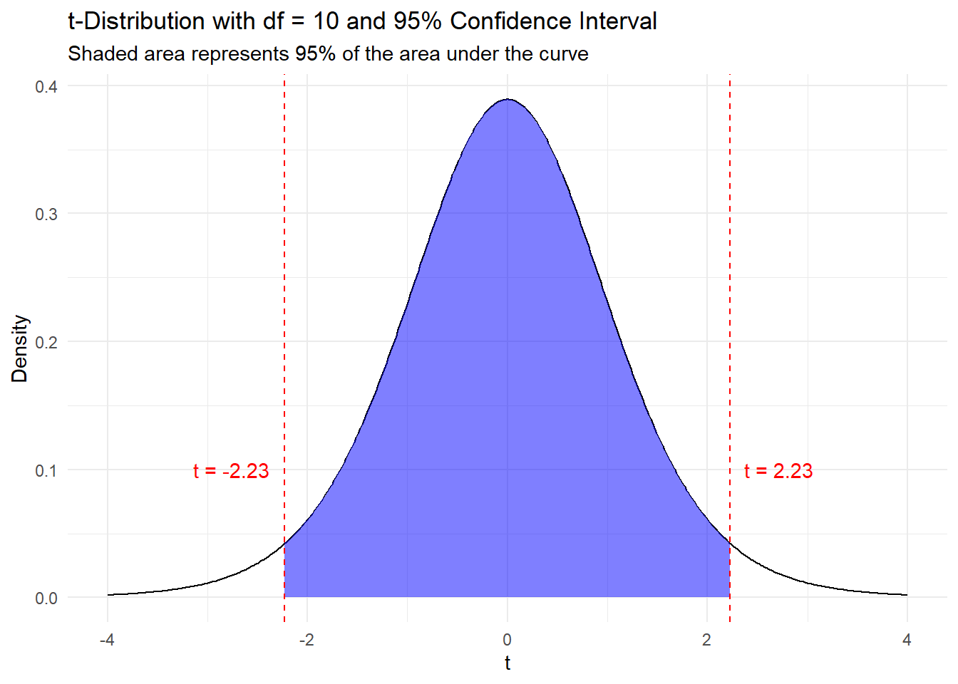
The critical value for the t-distribution is determined by the confidence level and the degrees of freedom. This is calculated by finding the value of \(t_{\alpha/2, df}\) such that the area under the t-distribution curve (with that specific degrees of freedom) between \(-t_{\alpha/2, df}\) and \(t_{\alpha/2, df}\) is equal to the confidence level.
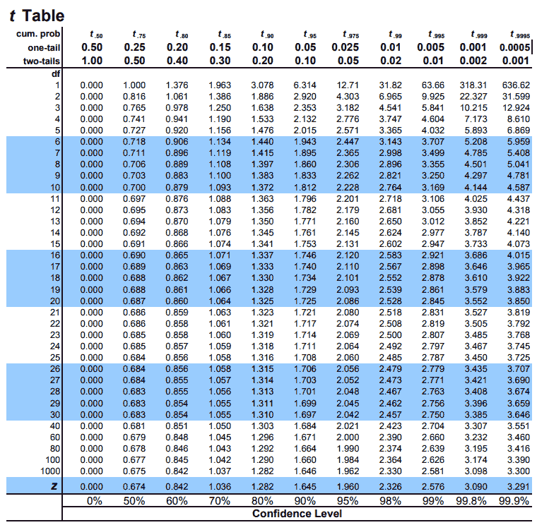
These critical values can be found using t-tables like the one below. Some important things to note about this specific t-table. The degrees of freedom for the test are on the left. The row cum. prob at the top shows us the \(t_{\alpha}\) value. The one-tail row shows us the p-value for a one-tailed test and the row two-tail shows us the p-value for a two-tailed test. There is also a helpful row at the bottom called confidence level that shows the associated confidence level for confidence intervals. The values in the table show the t-test statistic values corresponding to the degrees of freedom and \(t_{alpha}\).
For a 95% confidence interval, our Type I error rate is \(\alpha = 0.05\). Since confidence intervals are two-tailed, we split this \(\alpha\) in half, half in the left tail and half in the right tail. This means that we are looking for \(t_{.025, df}\) or \(t_{.975, df}\).
Example 1: t-distribution confidence intervals
We would like to make a 90% confidence interval for the true mean of scoring for Jon Rahm at the Masters. His scores were as follows.
| Golfer | Round | Score |
|---|---|---|
| Jon Rahm | 1 | 65 |
| Jon Rahm | 2 | 69 |
| Jon Rahm | 3 | 73 |
| Jon Rahm | 4 | 69 |
We start by calculating the the sample mean (\(\bar{x}\)).
\[ \begin{align*} \bar{x} &= \frac{65 + 69 + 73 + 69}{4} \\ &= 69 \end{align*} \]
Next we calculate the sample standard deviation (\(s\)).
\[ \begin{align*} s &= {\sqrt {\frac {\sum _{i=1}^{n}(x_{i}-{\overline {x}})^{2}}{n-1}}} \\ &= {\sqrt {\frac{(65 - 69)^2 + (69 - 69)^2 + (73 - 69)^2 + (69 - 69)^2}{4-1}}} \\ &= {\sqrt {\frac{(-4)^2 + 0^2 + 4^2 + 0^2}{3}}} \\ &\approx 3.266 \end{align*} \]
Our next step is to find the critical value for a 90% confidence interval with 3 degrees of freedom (\(t_{\alpha/2, df}\). We’ll use the t-table from earlier to find this.
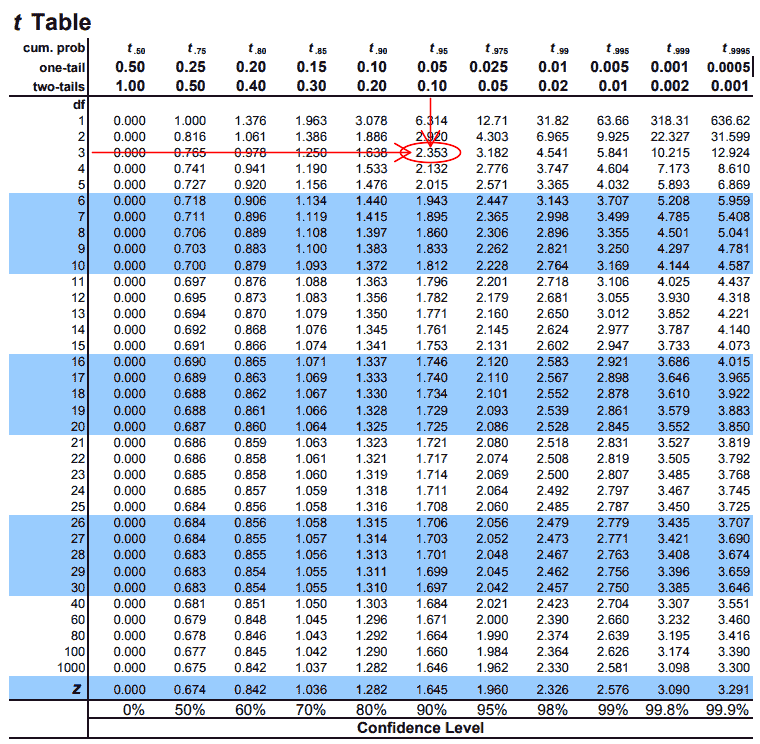
Lastly we will use the confidence interval formula to find the bounds of our 90% confidence interval. \[ \begin{align*} CI &= \bar{x} \pm t_{\alpha/2, df} \times \frac{s}{\sqrt{n}} \\ CI &= 69 \pm 2.353 \times \frac{3.266}{\sqrt{4}} \\ CI &= (67.07878, 70.92122) \end{align*} \] Finally we can interpret the confidence interval and say that we are 95% confident that the true mean of Jon Rahm’s scores at Augusta National is between 67.1 and 70.9.
TIP: When interpreting a confidence interval do not say “there is a 90% chance that the true mean is between the lower and upper bounds”. Instead, say “we are 90% confident that the true mean is between the lower and upper bounds”.
TIP: The t-table from earlier in the lesson will need to be used to find the critical value for the t-distribution for a 99% confidence interval with 6 degrees of freedom.
z-interval for single means
A standard normal distribution (also known as a z-distribution) is used to calculate the confidence interval for a single mean if the sample size is large enough (greater than 30) or the population standard deviation is known. The first case is common as oftentimes samples are greater than 30. The second case is rare because it is uncommon to know the population standard deviation but not the population mean.
The formula for the confidence interval for a single mean using the z-distribution is very similar to that of the t-distribution
Click here for more information about the standard normal distribution.
\(CI = \bar{X} \pm Z_{\alpha/2} \times \frac{\sigma}{\sqrt{n}}\)
Where \(\bar{X}\) is once again the sample mean, \(Z_{\alpha/2}\) is the critical value for the standard normal distribution at the specified confidence level, \({\sigma}\) is the population standard deviation, and \(n\) is the sample size.
The reasoning behind why we can use the standard normal distribution when the sample is greater than 30 even if the population standard deviation is unknown is found in the Central Limit Theorem, which says that as the sample size increases, the sampling distribution of the sample mean approaches a normal distribution. This means that when the sample size is greater than 30 we can use the sample standard deviation to estimate the population standard deviation and create a confidence interval as seen below
\(CI = \bar{X} \pm Z_{\alpha/2} \times \frac{s}{\sqrt{n}}\)
Once again the critical value for the z-distribution is the value of \(Z_{\alpha/2}\) such that the area under the standard normal distribution curve between \(-Z_{\alpha/2}\) and \(Z_{\alpha/2}\) is equal to the confidence level.
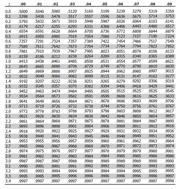
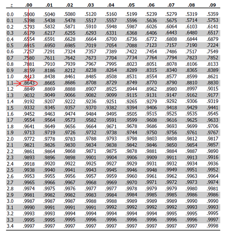
The critical values for the z-distribution can be found using a z-table such as the one below. All values in the table are the area under the standard normal curve to the left of the associated z-score. The column on the left shows the associated ones and tenths value for the z-score. The row at the top shows the associated hundredths value for the z-score.
Example 2: z-distribution confidence intervals
We would like to make a 98% confidence interval for the true mean of scoring for PGA Tour golfers based off of a sample from the third round. The sample includes the following scores.
Round 3 PGA Tour golfer scores: 73 76 71 75 70 73 71 72 71 74 73 68 74 67 73 73 70 72 74 74 69 73 74 74 72 78 74 76 74 72 77 70 74 77 72 73 74 74 77Whew! That’s 39 observations we have in our sample, which means we can use the z-distribution.
We start by calculating the the sample mean (\(\bar{x}\)). This probably has to be done using a calculator or programming tool. For this example our sample mean is approximately 73.03.
Next we calculate the sample standard deviation (\(s\)), which is our estimate for \(\sigma\). Once again, with a sample this size a calculator or computer is probably necessary for computing this. Our sample standard deviation is approximately 2.44.
Our next step is to find the critical value for a 98% confidence interval for a z-distribution (\(Z_{\alpha/2}\)). We will use the z-table from earlier. Since we want alpha equal to .2, our area to the right should be .1 and we look for the value on the table of .99.
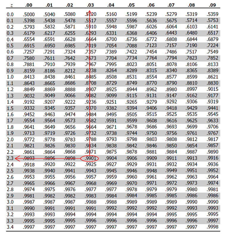
Note that this value is not exact. The value is slightly less than 2.33 but .9901 is closer to .99 than .9898, so we went with 2.33.
Lastly we will use the confidence interval formula to find the bounds for our 98% confidence interval. \[ \begin{align*} CI &= \bar{X} \pm Z_{\alpha/2} \times \frac{s}{\sqrt{n}} \\ CI &= 73.03 \pm 2.33 \times \frac{2.44}{\sqrt{39}} \\ CI &= (72.12, 73.94) \end{align*} \] Finally we can interpret the confidence interval and say that we are 98% confident that the true mean of PGA Tour golfers’ scores at the 2023 Masters is between 72.12 and 73.94.
Hypothesis Testing with Single Mean Confidence Intervals
Hypothesis testing is a method used to determine if a claim about a population parameter is true or not. In this section, we will perform the most common type of hypothesis test, a single mean test. The null hypothesis (\(H_0\)) is that the population mean is equal to a specific value, and the alternative hypothesis (\(H_a\)) is that the population mean is not equal to that value, greater than that value, or less than that value.
Null Hypothesis: \(H_0: \mu = \mu_0\)
Alternative Hypothesis Options:
\(H_a: \mu \neq \mu_0\) or
\(H_a: \mu > \mu_0\) or
\(H_a: \mu < \mu_0\)
Test Statistics
Like confidence intervals, we have two different tests for hypothesis testing for the population mean. Remember that if the population standard deviation is unknown and the sample size is less than 30, we use the t-distribution. If the population standard deviation is known or the sample size is greater than 30, we use the standard normal distribution.
Each of these distributions have their own tests, the t-test and the z-test. This means that we have different test statistics to calculate depending on the situation.
t-test
The t-test statistic is calculated using the formula:
\[t = \frac{\bar{x} - \mu_0}{\frac{s}{\sqrt{n}}}\]
where \(\bar{x}\) is the sample mean, \(\mu_0\) is the hypothesized population mean, \(s\) is the sample standard deviation, and \(n\) is the sample size.
z-test
The z-test statistic is calculated using the formula:
\[z = \frac{\bar{x} - \mu_0}{\frac{\sigma}{\sqrt{n}}}\]
where \(\bar{x}\) is the sample mean, \(\mu_0\) is the hypothesized population mean, \(\sigma\) is the population standard deviation, and \(n\) is the sample size.
Once again, if the sample size is over 30 and the population standard deviation is unknown, we use the sample standard deviation to approximate the population standard deviation.
To Reject or Fail to Reject
There are two ways to make a decision about the null hypothesis.
Method 1: Critical values, along with test statistics, can be used to determine if the hypothesized population mean is within the confidence interval for the true mean.
A critical value is a value that separates the rejection region from the non-rejection region. The rejection region is the area where the null hypothesis is rejected. The non-rejection region is the area where the null hypothesis is not rejected. The critical value is determined by the significance level (\(\alpha\)) and the degrees of freedom (if it is a t-test). The critical value is compared to the test statistic to determine if the null hypothesis should be rejected. If the test statistic is within the non-rejection region, the null hypothesis is not rejected. If the test statistic is within the rejection region, the null hypothesis is rejected and the alternative hypothesis is accepted.
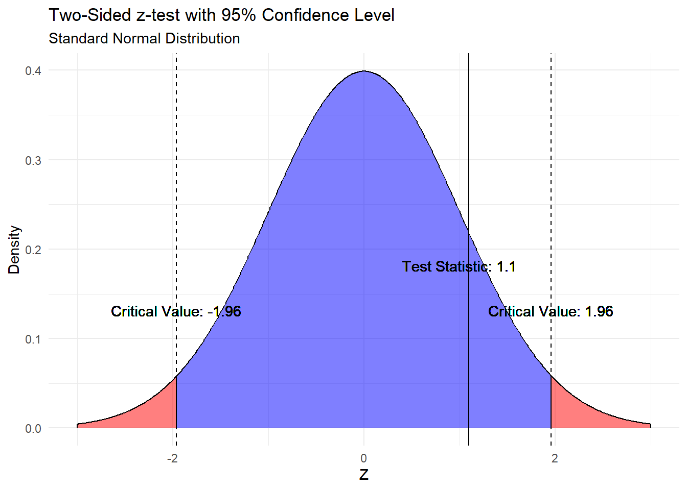
Below is an example of using critical values and a test-statistic for a z-test with a 95% confidence level (two-sided). The critical value is 1.96. This means that if the test statistic is greater than 1.96 or less than -1.96, the null hypothesis is rejected. The blue represents the non-rejection region and the red the rejection region. Since the test statistic for this example is 1.1 (less than 1.96 and greater than -1.96), we fail to reject the null hypothesis.
This method corresponds directly to the related confidence intervals produced for the sample data.
If the hypothesized population mean is within the confidence interval, we fail to reject the null hypothesis. If the hypothesized population mean is not within the confidence interval, the null hypothesis is rejected and the alternative hypothesis is accepted.
Note: We can say that there is significant evidence to accept the alternative hypothesis if the null hypothesis is rejected. However, it should never be said that we accept the null hypothesis. We can only fail to reject it.
Method 2: The second method is to use a p-value. The p-value is the probability of observing a test statistic as extreme as the one calculated from the sample data given that the null hypothesis is true. The p-value is compared to the significance level (\(\alpha\)) to determine if the null hypothesis should be rejected. If the p-value is less than \(\alpha\), the null hypothesis is rejected. If the p-value is greater than \(\alpha\), the null hypothesis is not rejected.
NOTE: Our alternative hypothesis determines whether we are looking for the probability that the test statistic is greater than or less than the observed value.
For a two-sided test, the p-value is the probability that the test statistic is greater than the observed value or less than the negative of the observed value. Find the area in one of the tails and double it.
For a left-tailed test (\(H_a: \mu < \mu_0\)), the p-value is the probability that the test statistic is less than the observed value.
For a right-tailed test (\(H_a: \mu > \mu_0\)), the p-value is the probability that the test statistic is greater than the observed value.
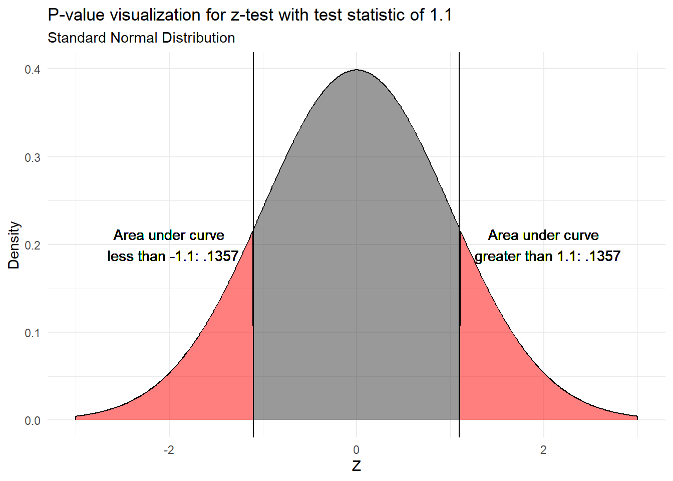
First let’s visualize what a p-value is telling us.
Now let’s see how we can calculate p-value for our example using a z-table.
We have a hypothetical z-test statistic of 1.1 and alpha of .05 for a two-tailed test. We start by finding the area under the curve to the left of a z-score of 1.1. However, we know that we want the area under the curve greater than 1.1 or less than -1.1. We can find the area under the curve to the right of 1.1 by subtracting our area value from 1. Additionally, we know that the z-distribution is symmetrical, implying that the area under the curve less than -1.1 is equal to that which is greater than 1.1. This means that we multiply our area value by 2 to get the p-value.
This means we can calculate p-value with the math below.
\[ \begin{align*} p\text{-}value &= 2 * (1 - .8643)\\ &= .2714 \end{align*} \]
Since the p-value is greater than our alpha value of .05 we fail to reject the null hypothesis.
Example 3: Hypothesis testing example
Suppose we have a sample of data with the following values: 10, 20, 30, 40, 50, 60, 70, 80, 90, 100. We want to test if the true mean of the population is not equal to 50. Alpha is 0.05. Our hypotheses are as follows:
- Null Hypothesis (\(H_0\)): \(\mu = 50\)
- Alternative Hypothesis (\(H_1\)): \(\mu \neq 50\)
We should use the t-test to test this hypothesis because the sample size is small and the population standard deviation is unknown.
We start by finding the sample mean, sample standard deviation, and degrees of freedom. Using a calculator we can find \(\bar{x} = 55\), \(s = 30.2765\), and logically \(df = 9\).
Now we need to find the critical value for a 95% two sided confidence t-interval with 9 degrees of freedom (\(t_{\alpha/2, df}\)). Once again we will use the t-table from earlier.
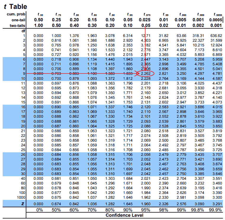
The critical value is \(\pm 2.262\).
Next the test statistic can be calculated as follows:
\[t = \frac{\bar{x} - \mu_0}{\frac{s}{\sqrt{n}}}\] \[t = \frac{55 - 50}{\frac{30.2765}{\sqrt{10}}}\] \[t = 0.522\]
This is visualized in the plot below.
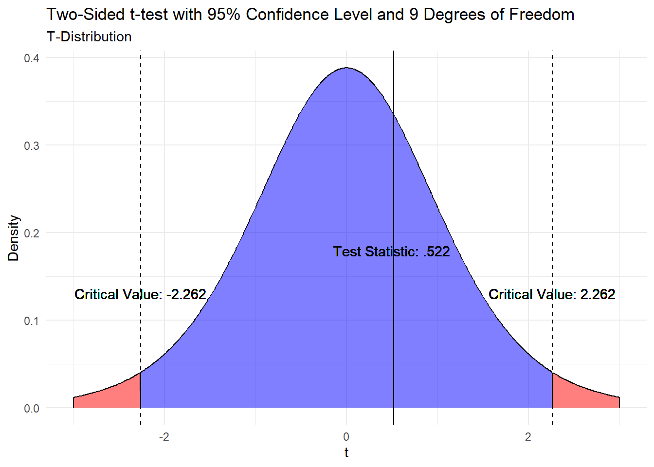
Since the test statistic is between the two critical values, there is not enough evidence to reject the null hypothesis and conclude that the true mean is not equal to 50.
The p-value for this example could be calculated by finding the area under the curve to the left of -0.522 and to the right of 0.522. The p-value would be the sum of these two areas.
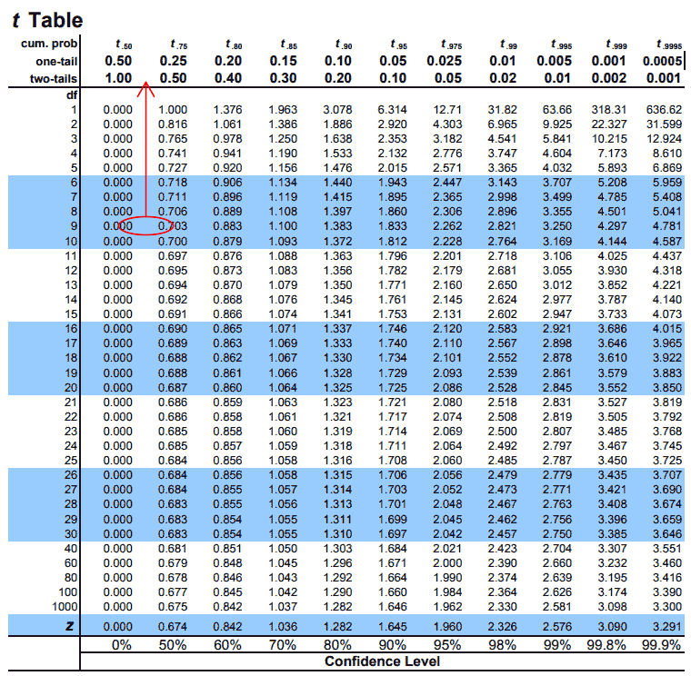
This value can be estimated by looking at the t-table. Obviously .522 is not on the table, but is between 0 and .703. If we follow this up to the top of the table we can look at the two-tails column and see that the p-value would be between .5 and 1. This is significantly larger than .05. Therefore we fail to reject the null hypothesis.
NOTE: Since this is a two-sided test you could simply find the probability that the test statistic is greater than 0.522 and multiply by 2. This would give you the p-value.
Hypothesizing Par as the Population Mean
Augusta National is breathtakingly beautiful, but if golfers get distracted by the scenic views, tall pines, bunkers, water, and azaleas may catch their balls.

Image Source: Your Golf Travel, CC 4.0
In golf par is considered to be the number of strokes a good golfer is expected to take. The par for the course at Augusta National is 72. It is known that Augusta National is a tougher than usual course, but we would like to test if that is the case for different groups of golfers.
Our null hypothesis will generally be that the true mean of the group is equal to 72.
Amateurs generally struggle in the Masters, but in 2023 Sam Bennett, a Texas A&M student, made the cut and finished 16th. However, due to his amateur status, he was not eligible to win money and missed out on $261,000.
More practice
If you would like more practice with confidence intervals and hypothesis testing, try the following exercises.
Fun fact: In the 2023 Masters Tournament, the average score for LIV golfers was just slightly worse (72.91) than the average score for PGA golfers (72.55). However, the average score for amateurs (74.56) and seniors (76.31) was significantly higher.
Think on it: The average score for the first 2 rounds of the 2023 Masters Tournament was 72.8, while the average score for the last 2 rounds was 73.22. This is interesting because only the top players make it to the last 2 rounds, so you would expect the scores to be lower. What could have changed so that the best players are now scoring worse?
Conclusion
In this module you have learned about single mean confidence intervals and single mean hypothesis tests. You have learned when to use a z-distribution and when to use a t-distribution. How to interpret p-values and confidence intervals was also covered.
With the Masters scoring data, you were able to calculate confidence intervals and test hypotheses about the mean score of different groups of golfers. We saw that in order to form confidence intervals for groups such as amateurs and seniors, we needed to use the t-distribution due to the small sample sizes. With larger sample sizes, such as the PGA golfers, we were able to use the z-distribution. These confidence intervals gave us a range of plausible values for the true mean score of each group. We also tested hypotheses about the mean scoring averages for PGA, LIV, and amateur golfers. We were able to make conclusions about the mean score of each group (whether or not that group’s mean was greater than or not equal to par) based on the test statistic and critical values or p-values.