| player | year | greens | holes | cut |
|---|---|---|---|---|
| Scottie Scheffler | 2023 | 247 | 416 | Other |
| Scottie Scheffler | 2023 | 657 | 760 | Fairway |
| Scottie Scheffler | 2023 | 28 | 48 | Bunker |
PGA - Scheffler Greens in Regulation (No R)
Sample Proportions
Single Proportion Confidence Intervals
Comparing Two Proportions
Exploring Probability Confidence Intervals with Golf Data
Welcome video
Introduction
In this module, you will be exploring the concept of confidence intervals for proportions through the lens of golf. Specifically, you will be analyzing the 2023 greens in regulation data for Scottie Scheffler. Scottie Scheffler was the number 1 ranked golfer in the world and the PGA Tour Player of the Year in 2023.
Getting started: Scottie Scheffler Greens data
The data shown below is what will be used for a majority of the lab. The data contains information about the number of greens hit in regulation by Scottie Scheffler in 2023 from different lies.
All data for the lab is from the PGA TOUR’s Website
You can view brief desciptions of the variables in the data by clicking the button below.
Terms to know
Before proceeding with the analysis, let’s make sure we know some golf terminology that will help us putt-putt our way through this lab.
Are greens in regulation important to scoring? Check out the table below to see how greens in regulation and lower handicaps go hand and hand
| Handicap | GIR % |
|---|---|
| 0 | 64% |
| 0-5 | 47% |
| 5-10 | 36% |
| 10-15 | 27% |
| 15-20 | 20% |
| 20-25 | 12% |
| 25-30 | 10% |
| 30+ | 6% |
Data Source: The Range by The Grint
A Par 3 hole should take 1 shot to reach the green in regulation 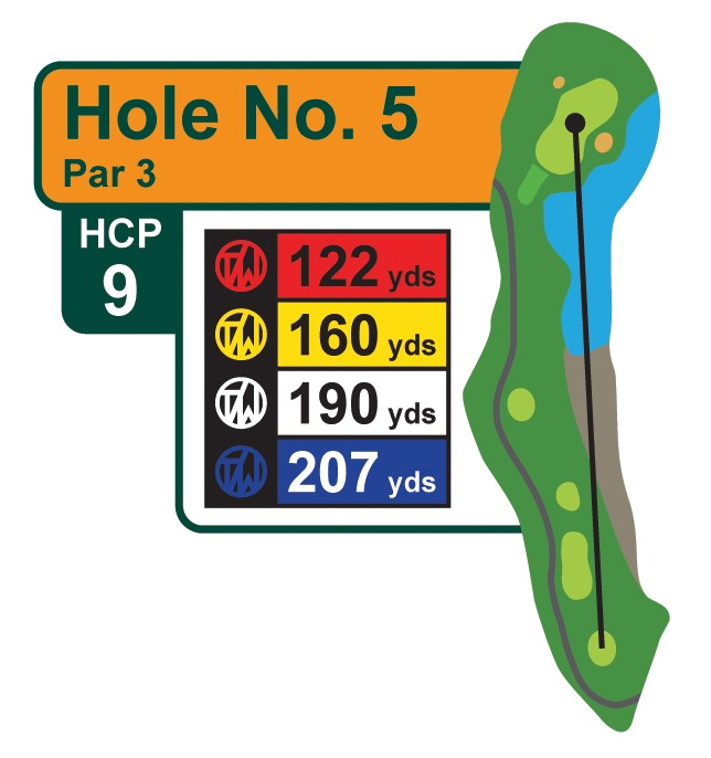
A Par 4 hole should take 2 shots to reach the green in regulation 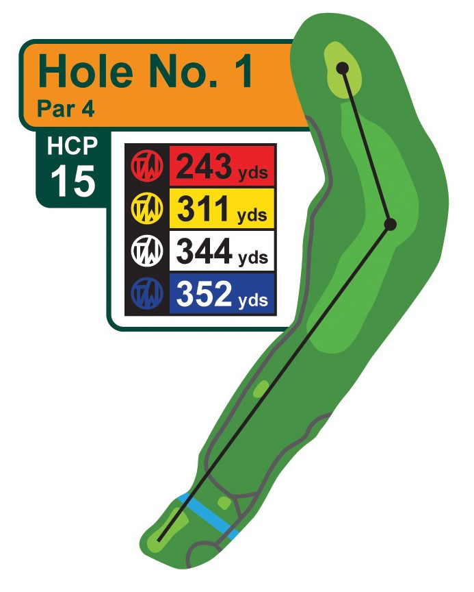
A Par 5 hole should take 3 shots to reach the green in regulation 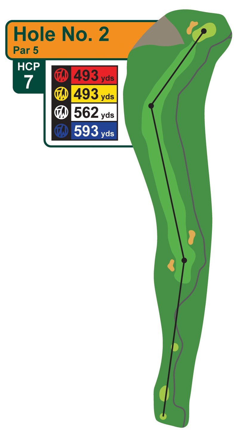 Images source: Tanglewood Golf Course, Public Domain
Lie Terminology
- The fairway is the short grass between the tee box and the green, where the ball is supposed to be hit on a par 4 or par 5 hole
- A bunker is a hazard filled with sand
- A fairway bunker is a bunker located in or next to the fairway
Sample Proportions
In statistics, a sample proportion (denoted \(\hat{p}\)) is an estimate of the true proportion of a population. The sample proportion is calculated by dividing the number of successes by the total number of observations in the sample.
The formula for the sample proportion is: \[\hat{p} = \frac{x}{n}\]
where \(x\) is the number of successes and \(n\) is the total number of observations in the sample.
Confidence Intervals for Proportions
A confidence interval for a proportion is a range of values that is likely to contain the true value of the population proportion with a certain level of confidence. Confidence intervals for proportions can be used for a variety of purposes, including:
Quantifying the precision of our estimates. The wider the confidence interval, the less precise our estimate is, the narrower the confidence interval, the more precise our estimate is.
Making inferences about the population proportion. For example, if a 90% confidence interval was used, it could be said that if the same population was sampled on numerous occasions and interval estimates were made on each occasion, approximately 90% of the intervals would contain the population parameter.
Testing hypothesized values of the population proportion. If the hypothesized value is not within the confidence interval, then we have reason to believe that it is not the true population proportion.
Comparing two proportions. If the confidence intervals for two sample proportions do not overlap, then we have reason to believe that the two true population proportions are different.
Making Confidence Intervals
The statistical notation for a confidence interval for a proportion is:
\[ \hat{p} \pm z \times \sqrt{\frac{\hat{p}(1-\hat{p})}{n}} \]
Where:
- \(\hat{p}\) is the sample proportion.
- \(z\) is the z-score that corresponds to the desired level of confidence
- \(n\) is the sample size
TIP: The z-score for a 95% confidence interval is approximately 1.96. You can use this value to calculate the confidence interval for the proportion of greens hit in regulation by Scottie Scheffler from the fairway.
Some common Confidence Intervals (two-sided) and their corresponding z-scores are:
| Confidence Interval | Z-Score |
|---|---|
| 90 % | 1.65 |
| 95 % | 1.96 |
| 98 % | 2.33 |
| 99 % | 2.58 |
For a quick example if the proportion of success for a problem is .6, the sample size is 100, and the test is being performed at the 95% confidence level, then the confidence interval for the proportion of success can be calculated as follows:
\[ \begin{align*} CI &= \hat{p} \pm z \times \sqrt{\frac{\hat{p}(1-\hat{p})}{n}} \\ CI &= .6 \pm 1.96 \times \sqrt{\frac{.6(1-.6)}{100}} \\ CI &= (.50398, .696102) \end{align*} \]
We are 95% confident that the true proportion of success is between .50398 and .696102.
Single Proportion Hypothesis Testing
Setting Up Hypotheses
In hypothesis testing for proportions, a null hypothesis is set up to test a claim about a population proportion. The null hypothesis is that the population proportion is equal to a specific value. The alternative hypothesis can be that the population proportion is not equal to the specific value, greater than the specific value, or less than the specific value.
The options are shown below:
NOTE: It is common practice to denote a null hypothesis with \(H_0\) and an alternative hypothesis with \(H_A\). Sometime the alternative hypothesis is denoted with \(H_1\).
\(H_0: p = p_0\)
and
\(H_A: p \neq p_0\) or
\(H_A: p > p_0\) or
\(H_A: p < p_0\)
Where \(p_0\) is the hypothesized value of the population proportion and \(p\) is the true population proportion.
Significance Level
For hypothesis testing, a significance level is set to determine the probability of rejecting the null hypothesis when it is true. The significance level is denoted by \(\alpha\) and is often set to 0.05. This means that there is a 5% chance of rejecting the null hypothesis when it is actually true. Other common significance levels are 0.01 and 0.10.
Calculating the Test Statistic
A test statistic is a value calculated from the sample data that is used to determine whether the null hypothesis should be rejected or not.
NOTE: The standard normal distribution is used to determine the critical value and test statistic for hypothesis testing for proportions. The standard normal distribution is a normal distribution with a mean of 0 and a standard deviation of 1. The distribution is symmetric about the mean and has a bell-shaped curve. The standard normal distribution is often called the z-distribution.
The test statistic for hypothesis testing for proportions is z, and the formula for it is as follows:
\[z = \frac{\hat{p} - p_0}{\sqrt{\frac{p_0(1 - p_0)}{n}}}\]
Where \(\hat{p}\) is the sample proportion, \(p_0\) is the hypothesized value of the population proportion, and \(n\) is the sample size.
Determining the Significance of the Test
There are two common ways to determine the significance of the test:
Compare the test statistic to the critical value
Compare the p-value to the significance level
The first method compares the test statistic to the critical value. The critical value is the value that separates the rejection region from the non-rejection region. If the test statistic is in the rejection region, the null hypothesis is rejected. This also corresponds to the confidence intervals given for the true probability of success. If the hypothesized value of the population proportion is within the confidence interval, the null hypothesis is not rejected. If it is outside the confidence interval, the null hypothesis is rejected.
The p-value is the most common way to determine the significance of the test. The p-value is the probability of observing a test statistic as extreme as the one calculated from the sample data, assuming the null hypothesis is true. If the p-value is less than the significance level, the null hypothesis is rejected.
TIP: Tables of z-scores and p-values like the one below can be used to determine the significance of the test. These tables show the area under the normal curve to the left of a given z-score.

Hypothesis Testing Example
Below is an example of hypothesis testing for proportions. First, we will set up the hypotheses:
\[H_0: p = 0.7\] \[H_A: p \neq 0.7\] The significance level is set to 0.05.
Our sample data has 60 successes out of 100 trials. The sample proportion is \(\hat{p} = 0.6\).
The test statistic is calculated as follows:
\[ \begin{align*} z &= \frac{0.6 - 0.7}{\sqrt{\frac{0.7(1 - 0.7)}{100}}} \\ z &= \frac{-0.1}{\sqrt{\frac{0.21}{100}}} \\ z &= \frac{-0.1}{0.045826} \\ z &= -2.183215 \end{align*} \]
Since alpha was set to 0.05, the critical value is \(\pm 1.96\). Since the test statistic is less than -1.96, the null hypothesis is rejected.
If we wanted to find the p-value, we would look up the z-score in a z-table. The area under the normal curve to the left of -2.183215 is 0.0146. Since this is a two-tailed test, the p-value is 0.0146 * 2 = 0.0292. Since the p-value is less than 0.05, the null hypothesis is rejected.
There is enough evidence to support the alternative hypothesis that the population proportion is not equal to 0.7.
Drawing Conclusions
If the null hypothesis is rejected we can conclude that the sample data provides enough evidence to support the alternative hypothesis. If the null hypothesis was that the population proportion is equal to .7 and the alternative hypothesis was that the population proportion is not equal to .7 and \(\alpha = 0.5\), then we might say,
“There is significant evidence to suggest that the true population proportion is not equal to .7 at the 95% confidence level.”
If the null hypothesis is not rejected we do not automatically accept the null hypothesis. We simply do not have enough evidence to reject it. For example, if the null hypothesis was that the population proportion is equal to .7 and the alternative hypothesis was that the population proportion is not equal to .7 and \(\alpha = .05\), then we might say,
There is not enough evidence to suggest that the true population proportion is different from .7 at the 95% confidence level.”
Testing a Hypothesized Proportion
Suppose you are watching a golf tournament on TV and Scottie Scheffler is about to hit an approach shot from the fairway. You hear the announcer say that Scottie Scheffler hits 3/4 of his greens in regulation from the fairway. You are skeptical of this claim and decide to test it against the data you have collected at the 95% confidence level.
You set up a hypothesis test with the following hypotheses:
Null Hypothesis \(H_0\): The proportion of greens hit in regulation by Scottie Scheffler from the fairway is 0.75.
Alternative Hypothesis \(H_A\): The proportion of greens hit in regulation by Scottie Scheffler from the fairway is not 0.75.
Two Sample z-test for Proportions
Sometimes, comparing two sample proportions is necessary to determine if they are significantly different. This can be done with a two sample z-test for equality of proportions.
The null hypothesis for a two sample z-test for equality of proportions is that the two proportions are equal.
\(H_0: p_1 = p_2\)
The alternative hypothesis can be that the two proportions are not equal, that the first proportion is greater than the second proportion, or that the first proportion is less than the second proportion. The options for the alternative hypothesis are shown below:
\(H_A: p_1 \neq p_2\)
\(H_A: p_1 > p_2\)
\(H_A: p_1 < p_2\)
The test-statistic for the two sample z-test for equality of proportions is calculated as:
\[Z = \frac{\hat{p}_1 - \hat{p}_2}{\sqrt{\hat{p}(1-\hat{p})\left(\frac{1}{n_1} + \frac{1}{n_2}\right)}}\]
where
\(\hat{p}_1\) and \(\hat{p}_2\) are the sample proportions for the two samples,
\(\hat{p}\) is the pooled proportion,
\(n_1\) and \(n_2\) are the sample sizes for the two samples.
The pooled proportion is calculated as:
\[\hat{p} = \frac{x_1 + x_2}{n_1 + n_2}\]
Comparing Two Proportions Example
Suppose you collect two samples of greens hit in regulation by two different golfers. Golfer A hits 10 out of 100 greens in regulation, while Golfer B hits 20 out of 100 greens in regulation. You want to test if the two golfers have significantly different greens hit in regulation at the 95% confidence level.
The hypotheses for the test are: \[H_0: p_1 = p_2\] \[H_A: p_1 \neq p_2\]
The test statistic is calculated as follows:
\[ \begin{align*} z &= \frac{\hat{p}_1 - \hat{p}_2}{\sqrt{\hat{p}(1-\hat{p})\left(\frac{1}{n_1} + \frac{1}{n_2}\right)}} \\ z &= \frac{0.1 - 0.2}{\sqrt{0.15(1 - 0.15)\left(\frac{1}{100} + \frac{1}{100}\right)}} \\ z &= \frac{-0.1}{\sqrt{0.15(0.85)\left(0.02\right)}} \\ z &= \frac{-0.1}{\sqrt{0.00255}} \\ z &= \frac{-0.1}{0.05050} \\ z &= -1.98030 \end{align*} \]
Since alpha was set to 0.05, the critical value is \(\pm 1.96\). Since the test statistic is less than -1.96 (just barely), the null hypothesis is rejected. There is enough evidence to support the alternative hypothesis that the two golfers have significantly different greens hit in regulation proportions.
Learn about rules about hitting out of the bunkers in golf in the video below:
TIP: When the alternative hypothesis is that the proportion from the first sample is greater than the proportion from the second sample, the test is a one-tailed test, meaning all of the error is in one tail of the distribution. This also means that the critical value of a one-tailed test at the 95% confidence level is the same as a two-tailed test at the 90% confidence level.
More Practice
Rory McIlroy is one of the most popular and best golfers on the PGA Tour. He has won multiple major championships. He is known for his long drives and his picturesque swing.

Image Source: TourProGolfClubs, CC BY 2.0, via Wikimedia Commons
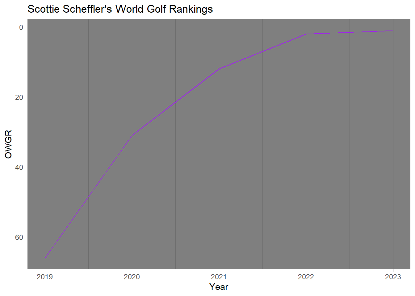
Below is a graph of Scottie Scheffler’s rapid climb up the world golf rankings from the end of 2019 to the end of 2023.
Conclusion
Conclusion
In this module you have learned how to calculate a sample proportion, form confidence intervals, conduct hypothesis tests, and compare proportions. You also learned how to interpret the results of these intervals and tests correctly. The effects of sample size and confidence level were also looked at in this module.
With the golf data we determined that Scottie Scheffler is better at hitting greens in regulation from the fairway than not in the fairway. We also saw that at times the difference in the sample proportions of greens hit in regulation between golfers or cuts was not significant enough to reject the claim that they are equal. When performing multiple tests at different significance levels, we sometimes got different results, proving the importance of choosing a significance level before conducting a test.