Lab 04 - National Women’s Soccer

Data wrangling

Joins

Sports analytics

National Women’s Soccer League

Goals

In this lab, you will:

Develop proficiency with data-wrangling functions
Join multiple datasets from the National Women’s Soccer League
Use wrangling and visualization to answer questions about team and player performance for the Portland Thorns FC

Joins allow us to combine information from multiple data sources into a single analytical workflow.

Getting Started

You will be working in your Lab 03–04 Groups (see Blackboard).
Download the .qmd file for this lab from our class GitHub repo.
Refer back to Lab 01 for detailed workflow and submission instructions.

Packages

We will primarily use the tidyverse package. Additional packages provide color palettes, table formatting, ridge plots, and access to NWSL data.

library(tidyverse)
library(viridis)
library(kableExtra)
library(ggridges)
library(devtools)
devtools::install_github("nwslR/nwslR", ref = "v0.0.0.9002")
library(nwslR)

Data: The Portland Thorns FC

For this lab, you will work with data about the Portland Thorns FC, a National Women’s Soccer League (NWSL) team.

In 2021, the Thorns won the:

NWSL Challenge Cup
Women’s International Champions Cup
NWSL Shield

The data come from the nwslR package, which provides tools to scrape and organize publicly available NWSL data.

The following functions pull different types of data:

load_matches() – match-level data
load_players() – player-level data
load_teams() – team information
load_metrics() – metric definitions

Running the code below will load four datasets into your environment.

matches <- load_matches()
players <- load_players()
teams   <- load_teams()
metrics <- load_metrics()

Exercises

All plots should follow best visualization practices discussed in lecture, including clear titles, labeled axes, and thoughtful aesthetic choices.

All code should follow the tidyverse style guidelines.

Data Wrangling

Before beginning the analysis, you will need to wrangle the data to focus only on Portland Thorns matches.

Exercise 1

Inspect the teams data to determine the external_team_id for the Portland Thorns.
Filter matches to keep only games in which Portland played (as the home or away team).
Save the result as portland_matches.

Confirm that the dataset has 223 observations before proceeding.

To add team names and abbreviations, we need to join the teams data twice:

once for the home team
once for the away team

We want the following new variables:

home_team_name
home_team_abbr
away_team_name
away_team_abbr

The code below creates home_team_info and joins it to portland_matches.

home_team_info <- teams |> 
  select(home_team_id = external_team_id,
         home_team_name = team_name,
         home_team_abbr = team_abbreviation)

portland_matches <- portland_matches |> 
  left_join(home_team_info)

Joining with `by = join_by(away_team_id)`

Exercise 2

Include the code above in your lab.
Then create an analogous away_team_info dataset with an away_ prefix and join it to portland_matches.

Confirm the dimensions are 223 × 19 before continuing.

Exercise 3

Create three new variables:

POR_points
OPP_points
result (Win, Loss, or Tie for Portland)

Use the scaffold below and fill in the blanks.

___ <- ___ |> 
  ___(POR_points = if_else(home_team_abbr == "POR",
                           home_team_score, away_team_score),
      OPP_points = if_else(___ ___ ___, ___, ___),
      result = case_when(POR_points  >  OPP_points ~ "Win",
                         POR_points  <  OPP_points ~ "Loss",
                         POR_points == OPP_points ~ "Tie"))

Match Analysis

Exercise 4

Create a bar chart showing the distribution of result.
Include clear axis labels and a title.
Interpret the results.

Exercise 5

Create a visualization examining Portland’s performance by season (wins, losses, and ties).
Describe 2–3 patterns you observe.

Exercise 6

Does Portland have a home-field advantage?

To investigate this question,

Create a variable indicating whether Portland was the home or away team
Make side-by-side boxplots of points scored
Create a ridge plot using geom_density_ridges()

Describe 2–3 observations.

Exercise 7

Create a formatted summary table showing the proportion of games won by whether the game was home or away.
Do the Thorns perform better at home or away?

Player Stats

The following code loads match-level player statistics. This step may take several minutes.

safe_load_pms <- purrr::possibly(load_player_match_stats,
                                 otherwise = data.frame())

player_stats <- purrr::map_df(portland_matches$match_id,
                              safe_load_pms,
                              .progress = TRUE)

In order to avoid loading the data everytime you render, add #| eval: false to the beginning of the above code chunk. After it has loaded, you can save the player_stats data by running saveRDS(player_stats, "data/player_stats.rds"). Then, include the following code in a new code chunk:

# Load saved version
# avoids lengthy re-loading from package on each Render
player_stats <- readRDS("./data/player_stats.rds")

The research questions:

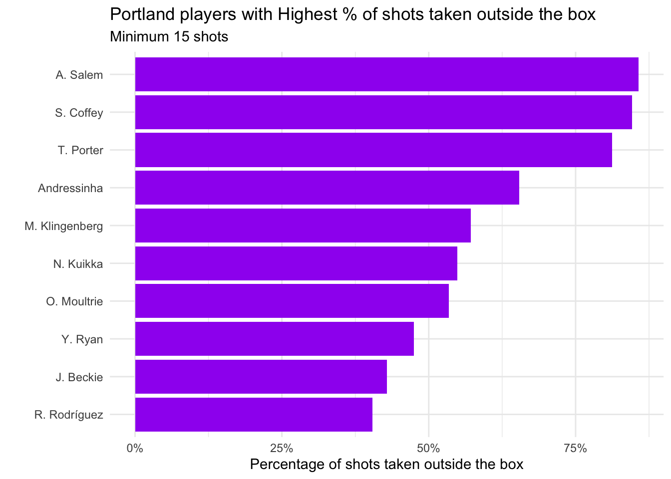
Which Portland players took the highest percentage of shots outside the box?
Which Portland players converted the highest percentage of shots?

Exercise 8

This is one big open-ended exercise to answer the two research questions above. It’s up to you to determine the appropriate wrangling necessary to answer the questions.

A few tips for getting started:

Examine player_stats using View() to determine what each row represents. Are there multiple rows per player? If so, what does each row represent?
You’ll only need theplayer_id, team_id, shots_total, shots_outside_box, and goals variables to answer these questions
Filter the data to only keep Portland players
Restrict your analysis to only players that took at least 15 shots across all matches
You will eventually need to join in info from the players data so that your end result will display the players names and not just their numerical id

Your final result for each question should be either a nicely formatted table, or a nicely formatted visualization, like the ones below. Use these end results to help you decide what wrangling will help you build up to this information.

player_match_name	shots_total	goals	prop_goals
E. Sonnett	26	8	0.3076923
H. Betfort	22	5	0.2272727
H. Sugita	47	10	0.2127660
T. Porter	16	3	0.1875000
N. Nadim	81	15	0.1851852
C. Sinclair	318	54	0.1698113
D. Brynjarsdóttir	41	6	0.1463415
H. Raso	97	13	0.1340206
A. Long	63	8	0.1269841
M. Purce	63	8	0.1269841

Bonus (2 pts)

Propose an additional question you could investigate using these data. Provide a visualization or table and briefly interpret the result.

Submission

Before submitting your .html:

Check code readability
Check visualization labels and titles
Ensure tables are cleanly formatted
Suppress unnecessary warnings and messages
Clearly label all exercises

Render one final time and submit the .html file to Blackboard.

Grading (50 pts)

Component	Points
Exercise 1	5
Exercise 2	5
Exercise 3	5
Exercise 4	5
Exercise 5	5
Exercise 6	5
Exercise 7	5
Exercise 8	10
Reflection	5